Lecture 1
Introduction and linear regression
How the course runs
Sessions
- 9 lectures of two hours
- 4 exercise sessions, after lectures 2, 4, 6 and 8
- A team project, on top of the exercises
Practicalities
- Exercises are Python notebooks that run in Google Colab: nothing to install
- Assessment: final exam 80%, team project assignment 20%
What the course covers
Learning from labelled examples
- Linear regression
- Polynomial regression and regularisation
- Classification and logistic regression
- Decision trees
Neural networks
- Neural networks 1
- Neural networks 2
- Convolutional networks
- Recurrent networks
Learning without labels
- Unsupervised learning
A first example: worn bearings
- Motors, pumps and wind turbines turn on rolling bearings
- A worn bearing vibrates more, and then fails
- A sensor on the housing records the vibration
The task
From a recording, decide whether the bearing is healthy or faulty.
Found early, a worn bearing is replaced at a planned stop, before it breaks the machine.
Programming versus learning
Programming
A person writes the rules.
rules + data → answers
If the vibration amplitude exceeds 7 mm/s, flag the bearing.
Machine learning
The computer finds the rules from examples.
data + answers → rules
Here are 10 000 recordings, each marked healthy or faulty.
A model you have probably used today
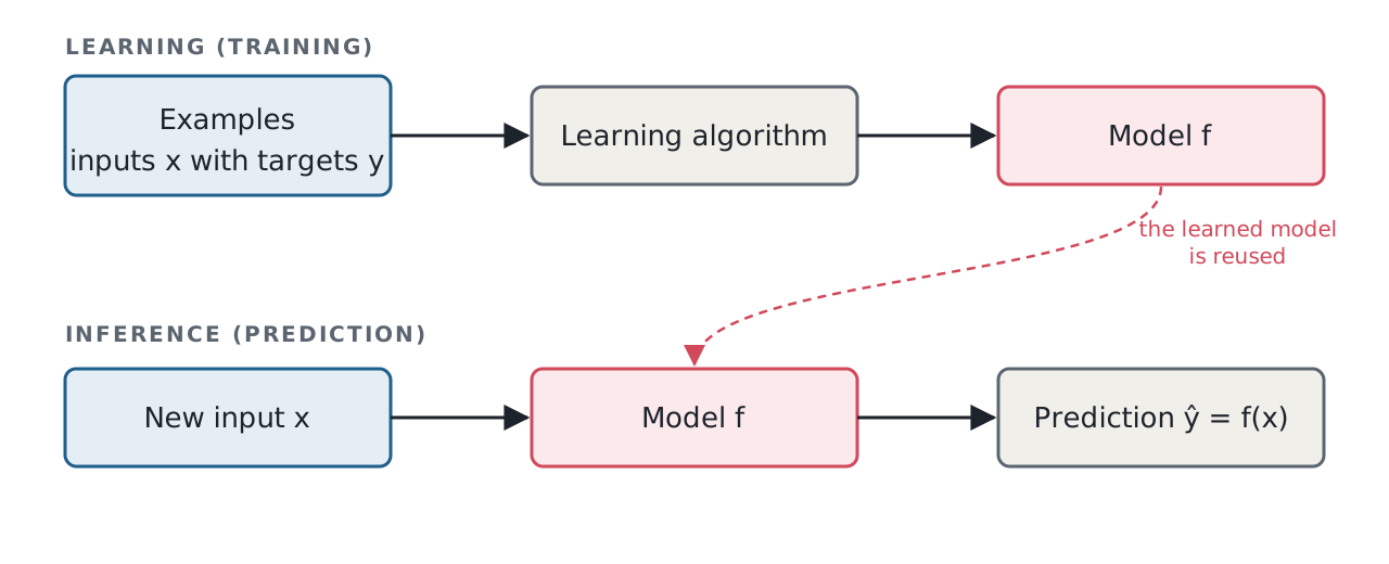
Learning
A language model reads billions of sentences and adjusts its parameters to predict the next word.
Inference
Given "The capital of Belgium is" it predicts "Brussels".
Same idea as this course, at a vastly larger scale: learn once, then predict many times.
Supervised learning in one picture
Checkpoint
Which of these are supervised learning problems?
- Predicting tomorrow's electricity load from past loads
- Grouping customers by their consumption profile, with no labels
- Detecting faulty bearings from vibration recordings labelled by technicians
Block 1
Data and features
The machine learning workflow
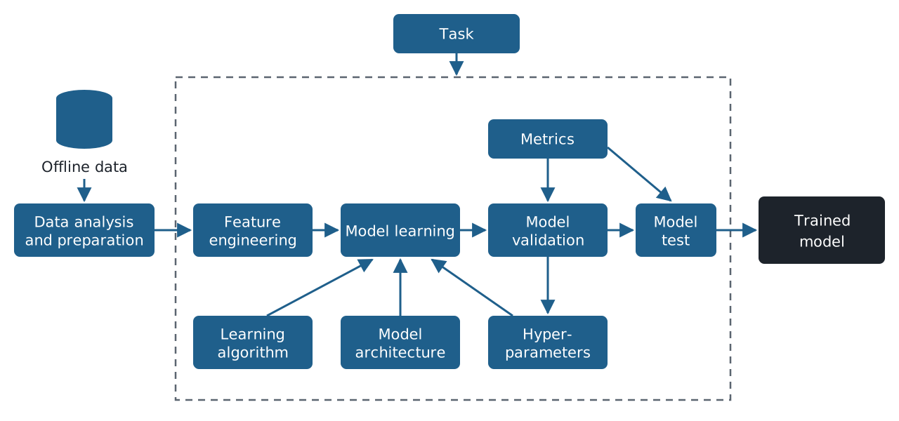
Samples, features and targets
A second example: wind turbines
| wind speed (m/s) | temperature (°C) | type | power (kW) |
|---|---|---|---|
| 4.2 | 11 | A | 85 |
| 7.9 | 9 | B | 610 |
| 12.5 | 14 | A | 2000 |
| 6.1 | 7 | C | 320 |
Predict the power a turbine delivers from the weather and its type.
One row is a sample \(\vx^{(i)} \in \R^d\).
One column is a feature \(x_j\).
The value to predict is the target \(y^{(i)}\).
\(n\) samples, \(d\) features.
Kinds of features
Numerical
- Continuous: wind speed, temperature
- Discrete: number of blades
Categorical
- Nominal, no order: turbine type A, B, C
- Ordinal, ordered: maintenance grade good < fair < poor
Everything becomes numbers
- An image: an array of pixel intensities
- A vibration signal: its samples, or its spectrum
- A text: word counts, or token numbers
The model only ever sees a vector
\[ \vx \in \R^d \]Choosing this representation is feature engineering, the second box of the workflow.
Encoding categories
Ordinal: keep the order
good → 0, fair → 1, poor → 2
Nominal: one-hot
| type | is A | is B | is C |
|---|---|---|---|
| A | 1 | 0 | 0 |
| B | 0 | 1 | 0 |
| C | 0 | 0 | 1 |
Regression and classification
Regression
The target is a number.
Power output in kW.
Classification
The target is a class.
Bearing healthy or faulty.
Today: regression. Lecture 3: classification.
Training data and test data
- The model learns from the training data
- Its quality is measured on test data it has never seen
- The test data are never used to make choices about the model
300 measurements: for example 240 for training and 60 for testing, split at random.
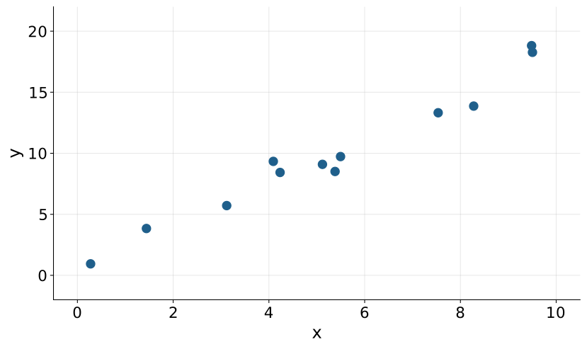
Fitting a line by eye
Which straight line fits these points best?
To answer, a number is needed that says how wrong a line is: a loss.
Checkpoint
Why not encode turbine type as 1, 2 and 3?
Block 2
Fitting a line
The model
- \(w_0\): intercept, \(w_1\): slope
- Every choice of \(\vw = (w_0, w_1)\) is one line
- Learning means choosing \(\vw\)
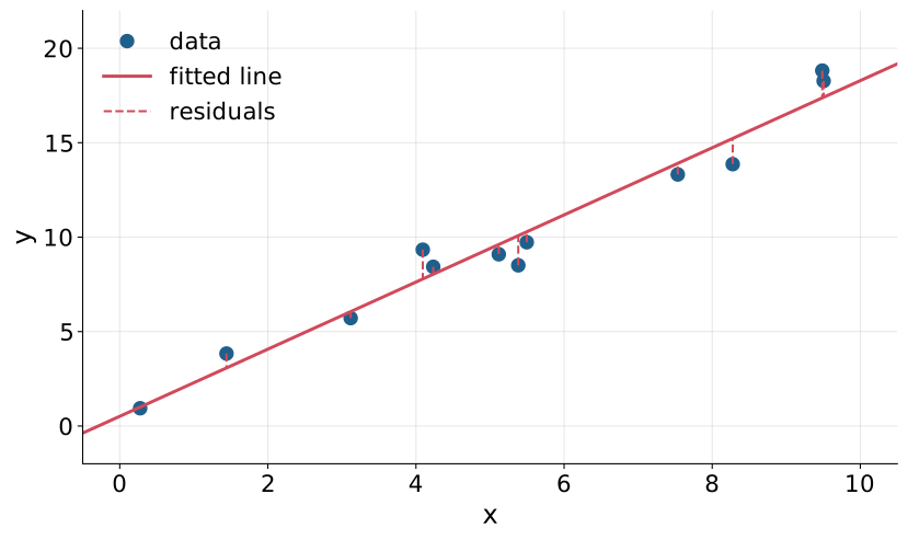
Residuals
For each sample, the error of the line:
\[ r^{(i)} = y^{(i)} - \yhat^{(i)} \]The dashed segments in the figure.
The loss: mean squared error
Squared: positive and negative errors do not cancel.
Squared: large errors weigh more than small ones.
Smooth, so it can be differentiated, which the next slides need.
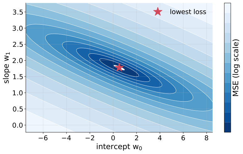
The loss as a landscape
- Every point is one line \((w_0, w_1)\)
- The height is the loss of that line
- Learning is finding the lowest point
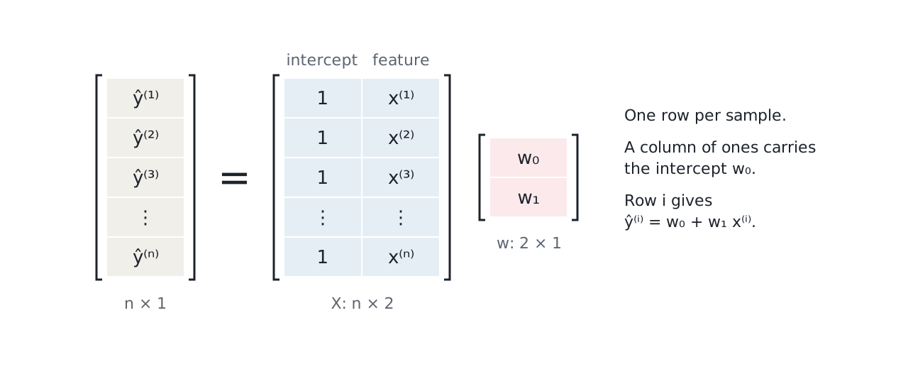
Writing it with matrices
The normal equations
At the bottom of a bowl the slope is zero in every direction.
What the normal equations need
- One exact step
- A \(d \times d\) system to solve: the cost grows like \(d^3\)
- An invertible \(\mX\T\mX\): duplicated features break it
An alternative that only needs the gradient: gradient descent.
Gradient descent: walk downhill
- The gradient points uphill, so step against it
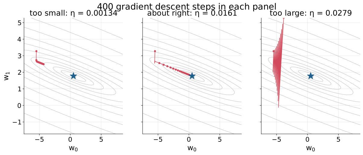
- \(\eta\) is the learning rate: the step size
In fog on a mountain: feel the slope under your feet, take a step down, repeat.
Gradient descent for linear regression
Pseudocode
input: X, y, learning rate η, steps T
w ← 0
repeat T times:
    g ← (2/n) Xᵀ (X w − y)
    w ← w − η g
return w
numpy
n = len(y)
w = np.zeros(X.shape[1])
for step in range(T):
    g = 2 / n * X.T @ (X @ w - y)
w = w - eta * gChoosing the learning rate
Two optimisers, one answer
| Normal equations | Gradient descent | |
|---|---|---|
| Steps | one | many |
| Cost | grows like \(d^3\) | cheap per step |
| Needs | invertible \(\mX\T\mX\) | a learning rate |
| Other losses | no | yes |
Both minimise the same loss, so both find the same \(\vw\).
Linear regression in three choices
Model
\(\yhat = \vw\T\vx\)
a straight line, a plane in more dimensions
Loss
\(\frac{1}{n}\sum_i \left(y^{(i)} - \yhat^{(i)}\right)^2\)
mean squared error
Optimiser
normal equations or gradient descent
solve exactly, or walk downhill
Checkpoint
Replace the squared error by the absolute error \(\lvert y - \yhat \rvert\). Which of the three choices changes, and can the normal equations still be used?
Break
Ten minutes
Block 3
More features, and how to judge a model
More than one feature
with \(x_0 = 1\) for the intercept.
- \(x_1\): wind speed
- \(x_2\): air density
- \(x_3\): temperature
The same formulas
- The design matrix gains one column per feature: \(n \times (d + 1)\)
- The normal equations do not change
- Gradient descent does not change
The matrix notation of block 2 pays off here.
Reading the weights
- \(w_j\): the change in \(\yhat\) per unit of \(x_j\), with the other features fixed
- Units matter: a weight per m/s cannot be compared with a weight per °C
Lecture 2 puts features on a common scale before comparing or penalising their weights.
Error in the units of the target
The MSE is in kW², which is hard to read. Its square root is in kW:
An RMSE of 120 kW means typical errors of about 120 kW.
The coefficient of determination
1: perfect predictions.
0: no better than always predicting the mean \(\bar{y}\).
Negative: worse than predicting the mean.
Training error and test error
- The training error is optimistic: the model has seen those points
- Report the error on the test data
Lecture 2: what happens to both errors when the model becomes very flexible.
What can go wrong: outliers
- One faulty sensor reading produces a huge residual
- Squaring makes that residual dominate the loss
- The line tilts towards the outlier
Look at the data before fitting. Losses that grow more slowly than the square are less sensitive.
What can go wrong: correlated features
- Wind speed in m/s and in km/h as two features
- \(\mX\T\mX\) cannot be inverted
- Nearly correlated features: the predictions can be fine while the weights are meaningless
Lecture 2: regularisation stabilises the weights.
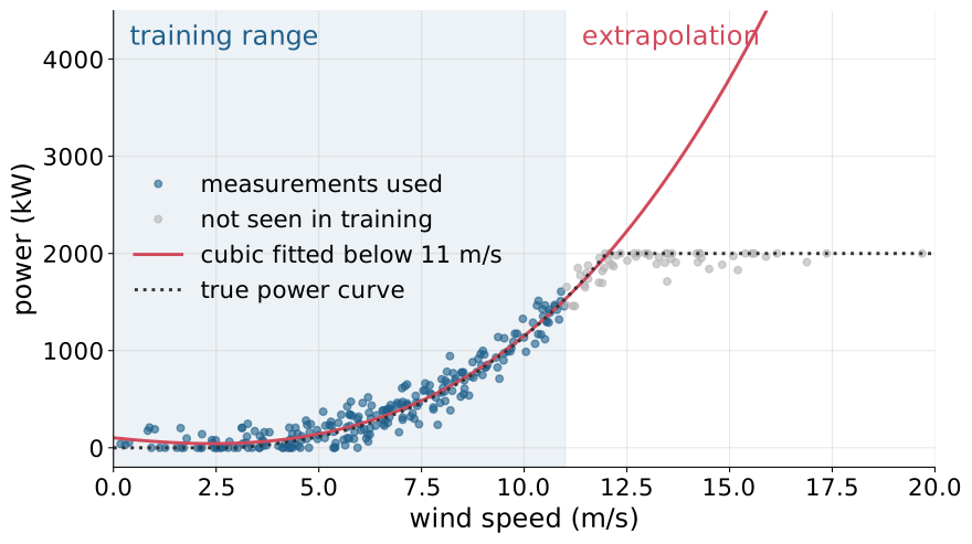
What can go wrong: extrapolation
A cubic fitted below 11 m/s keeps rising, while the turbine saturates at 2000 kW.
A model is only trusted inside the range of its training data.
Checkpoint
A model scores \(R^2 = 0.95\) on the training data and \(R^2 = 0.40\) on the test data. What happened, and which number do you report?
Takeaways
- Supervised learning builds a model from examples of inputs with known targets.
- Every method in this course is a choice of model, loss and optimiser.
- Linear regression: a linear model and the squared error, minimised exactly by the normal equations or step by step by gradient descent.
- The learning rate decides whether gradient descent crawls, converges or diverges.
- Judge a model on test data, and only trust it inside the range of its training data.
Nine lectures, three choices
Model
?
what shape of function
Loss
?
what counts as wrong
Optimiser
?
how we search
Further reading
- An Introduction to Statistical Learning with Applications in Python 2.1, 2.2, 3.1 to 3.3 The same least squares model, with the statistics behind it spelled out.
- The 100-page ML book 1, 2, 3.1, 4.1, 4.2 The vocabulary of this lecture in a few pages, useful before the next one.
- Understanding Deep Learning 2 Optional: the same supervised setup, written towards the networks of lecture 5.
All three books are free to read online.
Next
Lecture 2
Polynomial features, overfitting, validation and regularisation.
Exercise 1, after lecture 2
Regression on a wind turbine power curve, in numpy and scikit-learn.
Bring a laptop and a Google account for Colab.